General Usage
Import pygcc
from importlib.metadata import version
print(version("pygcc"))

from pygcc.pygcc_utils import *
1.5.3
Read database by specifying the direct- or sequential- access and source database
Using the default sequential-access database - speq21.dat
ps = db_reader(sourcedb = 'thermo.2021', sourceformat = 'gwb')
# ps.dbaccessdic, ps.sourcedic,  ps.specielist
Using the user-specified sequential-access database
ps = db_reader(dbaccess = './database/slop07.dat', sourcedb = 'thermo.2021', sourceformat = 'gwb')
# ps.dbaccessdic, ps.sourcedic,  ps.specielist
Duplicate found for species "AlOH++" in slop07.dat
Duplicate found for species "MgCO3(aq)" in slop07.dat
Duplicate found for species "CaCO3(aq)" in slop07.dat
Duplicate found for species "SrCO3(aq)" in slop07.dat
Duplicate found for species "BaCO3(aq)" in slop07.dat
Duplicate found for species "BaF+" in slop07.dat
Duplicate found for species "Sr(Succ)(aq)" in slop07.dat
Duplicate found for species "Sc(Glut)+(aq)" in slop07.dat
Duplicate found for species "AMP2-" in slop07.dat
Duplicate found for species "HAMP-" in slop07.dat
Duplicate found for species "+H2AMP-" in slop07.dat
Example: Calculate water properties
With IAPWS95
water = iapws95(T = np.array([  0.01, 25, 60,  100, 150,  200,  250,  300]), P = 200)
print('Density:', water.rho)
print('Gibbs Energy:', water.G)
print('Enthalpy:', water.H)
print('Entropy:', water.S)
Density: [1009.73580931 1005.83998999  991.7058825   967.43838406  927.69054221
  877.9652082   816.08878805  734.71208475]
Gibbs Energy: [-56194.26867312 -56592.33889817 -57211.87993461 -58000.04190115
 -59093.00868798 -60294.40876454 -61596.26593847 -62995.11966287]
Enthalpy: [-68680.33499723 -68236.29564253 -67613.18053963 -66897.34619192
 -65991.9279271  -65062.66635227 -64087.83220987 -63021.29280159]
Entropy: [15.14005087 16.69550855 18.67153539 20.7005717  22.97720284 25.05223509
 27.00976077 28.9549847 ]
With ZhangDuan
water = ZhangDuan(T= np.array([1000, 1050]), P = np.array([1000, 2000]))
print(water.rho, water.G)
[175.8286937 314.74510733] [-88767.03099 -89082.94223142]
Example: Calculate water dielectric constants
dielect = water_dielec(T= np.array([1000, 1050]), P = np.array([1000, 2000]), Dielec_method = 'DEW')
dielect.E, dielect.rhohat, dielect.Ah, dielect.Bh
(array([1.19637079, 2.52660344]),
 array([0.17582869, 0.31474511]),
 array([12.8720893 ,  5.29642074]),
 array([0.5403405 , 0.48797969]))
dielect = water_dielec(T= np.array([100, 150]), P = np.array([100, 200]), Dielec_method = 'JN91')
dielect.E, dielect.rhohat, dielect.Ah, dielect.Bh
(array([55.83017195, 44.79388023]),
 array([0.96293375, 0.92769054]),
 array([0.59551378, 0.67352582]),
 array([0.34191435, 0.35183609]))
Example: Calculate quartz properties
With Maier-Kelly powerlaw
Temp = np.array([100, 200, 400, 600, 800, 900])
ps = db_reader()
sup = heatcap( T = Temp, P = 1, Species = 'Quartz', Species_ppt = ps.dbaccessdic['Quartz'],
             method = 'SUPCRT')
sup.dG, sup.dCp
(array([-205319.43164294, -206728.65136032, -210399.56629393,
        -215044.47020067, -220518.04896025, -223492.57970966]),
 array([12.34074489, 13.89377788, 16.14397572, 16.103911  , 16.491911  ,
        16.685911  ]))
With Holland and Power’s formulation
Temp = np.array([100, 200, 400, 600, 800, 900])
pshp = db_reader(dbHP_dir = './database/supcrtbl.dat')
hp = heatcap( T = Temp, P = 10, Species = 'Quartz', Species_ppt = pshp.dbaccessdic['Quartz'],
             method = 'HP11')
hp.dG, hp.dCp
Duplicate found for species "Fluorphlogopite" in supcrtbl.dat
Duplicate found for species "Arsenic" in supcrtbl.dat
Duplicate found for species "Arsenolite" in supcrtbl.dat
(array([-205491.44716714, -206900.38310661, -210575.79120014,
        -215228.32290096, -220682.44526921, -223649.25812766]),
 array([12.4075447 , 13.99685509, 16.16426364, 16.05341748, 16.6660167 ,
        16.90252028]))
With Berman’s formulation
Temp = np.array([100, 200, 400, 600, 800, 900])
ps = db_reader(dbBerman_dir = './database/berman.dat')
bm = heatcap( T = Temp, P = 1, Species = 'Quartz', Species_ppt = ps.dbaccessdic['Quartz'],
             method = 'berman88')
bm.dG, bm.dCp
Duplicate found for species "Cordierite" in berman.dat
(array([-205498.95550508, -206907.11144614, -210575.29239247,
        -215221.44900321, -220654.77893829, -223612.45803826]),
 array([12.323813  , 13.87414095, 16.29997608, 16.24449507, 16.72930639,
        16.90352372]))
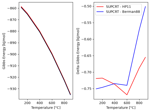
import matplotlib.pyplot as plt
fig, (ax1, ax2) = plt.subplots(1, 2)
ax1.plot(Temp, sup.dG*4.182/1e3, 'r', Temp, hp.dG*4.182/1e3, 'b', Temp, bm.dG*4.182/1e3, 'k')
ax1.set_xlabel('Temperature [°C]'); ax1.set_ylabel('Gibbs Energy [kJ/mol] ')
plt.legend(['SUPCRT', 'HP11', 'Berman88'])
ax2.plot(Temp, hp.dG*4.182/1e3 - sup.dG*4.182/1e3, 'r', Temp, bm.dG*4.182/1e3 - sup.dG*4.182/1e3, 'b')
ax2.set_xlabel('Temperature [°C]'); ax2.set_ylabel('Delta Gibbs Energy [kJ/mol] ')
plt.legend(['SUPCRT - HP11', 'SUPCRT - Berman88'])
fig.tight_layout()
Matplotlib is building the font cache; this may take a moment.
Example: Calculate olivine solid solutions
calc = calcRxnlogK( X = 0.85,T = np.array([300, 400, 450]), P = np.array([200, 200, 200]),
                   Specie = 'olivine', dbaccessdic = ps.dbaccessdic, densityextrap = True)
calc.logK, calc.Rxn
(array([ 9.2646654 , 23.54844166, 19.7311314 ]),
 {'type': 'ol',
  'name': 'Fo85',
  'formula': 'Mg1.70Fe0.30Si1O4',
  'MW': 150.1557,
  'min': ['Mg1.70Fe0.30Si1O4',
   ' R&H95, Stef2001',
   np.float64(-466862.12264868076),
   nan,
   np.float64(26.21037219328013),
   44.049,
   24.058078393881452,
   0.017393236137667304,
   -890893.8814531548,
   171.38145315487571,
   -3.6586998087954105e-06],
  'spec': ['H+', 'Mg++', 'Fe++', 'SiO2(aq)', 'H2O'],
  'coeff': [-4, 1.7, 0.30000000000000004, 1, 2],
  'nSpec': 5,
  'V': 44.049,
  'source': ' R&H95, Stef2001',
  'elements': ['1.7000', 'Mg', '0.3000', 'Fe', '1.0000', 'Si', '4.0000', 'O']})
Example: Calculate glauconite mineral properties
Temp = np.array([0.01, 20, 30, 40, 60, 80, 100, 150])
calc = calcRxnlogK(T = Temp, P = 'T', Specie = 'clay', dbaccessdic = ps.dbaccessdic, densityextrap = True,
                   elem = ['Glauconite', '3.654', '.687', '1.175', '0.079', '0.337', '0.679', '0.212', '0.0359', '0'])
calc.logK, calc.Rxn
(array([ 7.33889672,  6.08136856,  5.34485756,  4.59351803,  3.11784876,
         1.73061272,  0.45134995, -2.30826164]),
 {'type': 'Smectite',
  'name': 'Glauconite',
  'formula': 'K0.68Na0.21Fe0.08Ca0.04Mg0.34Al0.69FeIII1.18Si3.654O10(OH)2',
  'MW': 426.25271512,
  'min': ['K0.68Na0.21Fe0.08Ca0.04Mg0.34Al0.69FeIII1.18Si3.654O10(OH)2',
   'B2015, B2021',
   np.float64(-1173001.1408482206),
   np.float64(-1256479.2241755025),
   np.float64(90.78782850627151),
   np.float64(141.34069593680297),
   np.float64(77.70879420984171),
   np.float64(83.36446524554509),
   np.float64(-17.841879278113826)],
  'struct_formula': '(K0.679Na0.212Ca0.036)(Mg0.337Fe0.079Al0.341FeIII1.175)(Si3.654Al0.346)O10(OH)2',
  'spec': ['H+',
   'K+',
   'Na+',
   'Fe++',
   'Ca++',
   'Mg++',
   'Al+++',
   'Fe+++',
   'SiO2(aq)',
   'H2O'],
  'coeff': [np.float64(-7.381),
   0.679,
   0.212,
   0.079,
   0.0359,
   0.337,
   0.687,
   1.175,
   3.654,
   4.692],
  'nSpec': 10,
  'V': np.float64(141.34069593680297),
  'dG': np.float64(-4907.836773308955),
  'dHf': np.float64(-5257.109073950302),
  'S': np.float64(379.85627447024),
  'Cp': 345.17439398884756,
  'source': 'B2015, B2021',
  'elements': ['0.0359',
   'Ca',
   '0.6790',
   'K',
   '0.2120',
   'Na',
   '1.2540',
   'Fe',
   '0.3370',
   'Mg',
   '0.6870',
   'Al',
   '3.6540',
   'Si',
   '2.0000',
   'H',
   '12.0000',
   'O']})
Example: Create new reactions and calculate equilibrium constants
An example with pyrite, pyrrhotite, magnetite (PPM) reaction
Pyrite + 4 H2O + 2 Pyrrhotite → 4 H2S(aq) + Magnetite
Then we can include the reaction in sourcedic, one of the output of db_reader, which is a dictionary of list of reaction coefficients and species. An example with the format for sourcedic is as follows:
ps.sourcedic[‘Name’] = [‘formula’, number of reactants in the reaction, ‘coefficient of specie 1’, ‘specie 1’, ‘coefficient of specie 2’, ‘specie 2’]
AB → 0.5 A2(aq) + B
ps.sourcedic[‘AB’] = [‘AB’, 2, ‘0.5’, ‘A2(aq), ‘1’, ‘B’]
ps = db_reader(sourcedb = './database/thermo.2021.dat', sourceformat = 'gwb')
ps.sourcedic['Pyrite'] = ['', 4, '4', 'H2S(aq)', '1', 'Magnetite',  '-2', 'Pyrrhotite', '-4', 'H2O']
Temp = np.array([300.0000, 325, 350.0000, 400.0000, 415, 425.0000, 435, 450.0000])
Press = 500*np.ones(np.size(Temp))
log_K_PPM = calcRxnlogK( T = Temp, P = Press, Specie = 'Pyrite', dbaccessdic = ps.dbaccessdic,
                        sourcedic = ps.sourcedic, specielist = ps.specielist).logK
log_K_PPM
array([-9.61842122, -8.38742387, -7.21969753, -4.97772897, -4.29319566,
       -3.81890541, -3.32234015, -2.52289322])
Example: Generate GWB thermodynamic database
Note: GWB requires exactly 8 temperature and pressure pairs
# Vectors for Temperature (C) and Pressure (bar) inputs
T = np.array([  0.010,   25.0000 ,  60.0000,  100.0000, 120.0000,  150.0000,  250.0000,  300.0000])
P = 350*np.ones(np.size(T))
nCa = 1
write GWB using default sourced database, with inclusion of solid_solution and clay thermo properties
%%time
write_database(T = T, P = P, cpx_Ca = nCa, solid_solution = 'Yes',  clay_thermo = 'Yes',
               dataset = 'GWB')
Success, your new GWB database is ready for download
Database for GWB generated successfully using JN91 dielectric constant, thermo.com.tdat GWB source database, full solid solution included, clay thermodynamics included
  Supplemental built-in thermodynamic data: Ankerite [H&P2011               31.DEC.11]; Fluorapatite [R&H95]
CPU times: user 4.24 s, sys: 89.4 ms, total: 4.33 s
Wall time: 4.26 s
<pygcc.pygcc_utils.write_database at 0x7e0698dda990>
write GWB using user-specified sourced database, with inclusion of solid_solution and clay thermo properties
%%time
src_db = os.path.join(os.getcwd(), 'database', 'thermo.29Sep15.dat')
write_database(T = T, P = 175, cpx_Ca = nCa, solid_solution = 'Yes', clay_thermo = 'Yes',
                sourcedb = src_db, dataset = 'GWB')
Success, your new GWB database is ready for download
Database for GWB generated successfully using JN91 dielectric constant, thermo.29Sep15.dat GWB source database, full solid solution included, clay thermodynamics included
CPU times: user 3.64 s, sys: 104 ms, total: 3.74 s
Wall time: 3.63 s
<pygcc.pygcc_utils.write_database at 0x7e06912ee390>
write GWB using Jan2020/Apr20 formatted sourced database
%%time
src_db = os.path.join(os.getcwd(), 'database', 'thermo.com.tdat')
write_database(T = T, P = 125, cpx_Ca = nCa, solid_solution = True, clay_thermo = True,
                sourcedb = src_db, dataset = 'GWB')
Success, your new GWB database is ready for download
Database for GWB generated successfully using JN91 dielectric constant, thermo.com.tdat GWB source database, full solid solution included, clay thermodynamics included
  Supplemental built-in thermodynamic data: Fluorapatite [R&H95]
CPU times: user 4.27 s, sys: 119 ms, total: 4.39 s
Wall time: 4.27 s
<pygcc.pygcc_utils.write_database at 0x7e0698c372d0>
write GWB using Jan2020/Apr20 formatted sourced database with logK as polynomial coefficients, using Tmax and Tmin
%%time
src_db = os.path.join(os.getcwd(), 'database', 'thermo.com.tdat')
write_database(T = [0, 300], P = 150, clay_thermo = True, logK_form = 'polycoeffs',
               sourcedb =  src_db, dataset = 'GWB')
Success, your new GWB database is ready for download
Database for GWB generated successfully using JN91 dielectric constant, thermo.com.tdat GWB source database, clay thermodynamics included
  Supplemental built-in thermodynamic data: Fluorapatite [R&H95]
CPU times: user 3.46 s, sys: 10.7 ms, total: 3.47 s
Wall time: 3.47 s
<pygcc.pygcc_utils.write_database at 0x7e0698e75090>
write GWB using Mar21 formatted sourced database with logK as polynomial coefficients
%%time
src_db = os.path.join(os.getcwd(), 'database', 'thermo_latest.tdat')
write_database(T = [0, 300], P = 145, clay_thermo = True, logK_form = 'polycoeffs',
               sourcedb =  src_db, dataset = 'GWB')
Success, your new GWB database is ready for download
Database for GWB generated successfully using JN91 dielectric constant, thermo_latest.tdat GWB source database, clay thermodynamics included
  Supplemental built-in thermodynamic data: Fluorapatite [R&H95]
CPU times: user 3.38 s, sys: 17.4 ms, total: 3.4 s
Wall time: 3.39 s
<pygcc.pygcc_utils.write_database at 0x7e069080aa10>
write GWB using user-specified sourced database and direct-access database (slop07) and FGL97 dielectric constant
%%time
db_db = os.path.join(os.getcwd(), 'database', 'slop07.dat')
src_db = os.path.join(os.getcwd(), 'database', 'thermo.29Sep15.dat')
write_database(T = [0, 400], P = 300, cpx_Ca = 0.5, solid_solution = 'Yes', Dielec_method = 'FGL97',
                dbaccess = db_db,  sourcedb = src_db, dataset = 'GWB')
Duplicate found for species "AlOH++" in slop07.dat
Duplicate found for species "MgCO3(aq)" in slop07.dat
Duplicate found for species "CaCO3(aq)" in slop07.dat
Duplicate found for species "SrCO3(aq)" in slop07.dat
Duplicate found for species "BaCO3(aq)" in slop07.dat
Duplicate found for species "BaF+" in slop07.dat
Duplicate found for species "Sr(Succ)(aq)" in slop07.dat
Duplicate found for species "Sc(Glut)+(aq)" in slop07.dat
Duplicate found for species "AMP2-" in slop07.dat
Duplicate found for species "HAMP-" in slop07.dat
Duplicate found for species "+H2AMP-" in slop07.dat
Success, your new GWB database is ready for download
Database for GWB generated successfully using FGL97 dielectric constant, thermo.29Sep15.dat GWB source database, full solid solution included
CPU times: user 3.61 s, sys: 153 ms, total: 3.76 s
Wall time: 3.6 s
<pygcc.pygcc_utils.write_database at 0x7e06913087d0>
write GWB using default sourced database and direct-access database (slop07 with Berman mineral data) and FGL97 dielectric constant
%%time
db_berman = os.path.join(os.getcwd(), 'database', 'berman.dat')
db_db = os.path.join(os.getcwd(), 'database', 'slop07.dat')
write_database(T = [0, 340], P = 150, Dielec_method = 'FGL97',  dbaccess = db_db,
                dbBerman_dir = db_berman, dataset = 'GWB')
Duplicate found for species "AlOH++" in slop07.dat
Duplicate found for species "MgCO3(aq)" in slop07.dat
Duplicate found for species "CaCO3(aq)" in slop07.dat
Duplicate found for species "SrCO3(aq)" in slop07.dat
Duplicate found for species "BaCO3(aq)" in slop07.dat
Duplicate found for species "BaF+" in slop07.dat
Duplicate found for species "Sr(Succ)(aq)" in slop07.dat
Duplicate found for species "Sc(Glut)+(aq)" in slop07.dat
Duplicate found for species "AMP2-" in slop07.dat
Duplicate found for species "HAMP-" in slop07.dat
Duplicate found for species "+H2AMP-" in slop07.dat
Duplicate found for species "Cordierite" in berman.dat
Success, your new GWB database is ready for download
Database for GWB generated successfully using FGL97 dielectric constant, thermo.com.tdat GWB source database
  Supplemental built-in thermodynamic data: Fluorapatite [Berman_1988]; Ankerite [H&P2011               31.DEC.11]
CPU times: user 2.37 s, sys: 68.5 ms, total: 2.44 s
Wall time: 2.37 s
<pygcc.pygcc_utils.write_database at 0x7e069079e6d0>
write GWB using Mar21 formatted sourced database and direct-access database (speq21 with HP mineral data) and DEW dielectric constant
%%time
write_database(T = [0, 275], P = 1100, Dielec_method = 'DEW',  dbaccess = os.path.join(os.getcwd(), 'database', 'speq21.dat'),
                dbHP_dir = os.path.join(os.getcwd(), 'database', 'supcrtbl.dat'),
                sourcedb = os.path.join(os.getcwd(), 'database', 'thermo_latest.tdat'), dataset = 'GWB')
Duplicate found for species "Fluorphlogopite" in supcrtbl.dat
Duplicate found for species "Arsenic" in supcrtbl.dat
Duplicate found for species "Arsenolite" in supcrtbl.dat
/home/docs/checkouts/readthedocs.org/user_builds/pygcc/envs/latest/lib/python3.11/site-packages/pygcc/pygcc_utils.py:1984: UserWarning: Warning: Using SiO2(aq) data from Sverjensky et al. (2014) GCA. This thermodynamic model requires that you also add data for Si2O4(aq) to achieve accurate solubility calculations.Please ensure thermodynamic data for Si2O4(aq) are added to both your source GWB or EQ3/6 database AND your source direct-access database.
  warnings.warn(
Success, your new GWB database is ready for download
Database for GWB generated successfully using DEW dielectric constant, thermo_latest.tdat GWB source database
  Supplemental built-in thermodynamic data: Fluorapatite [ref:ZS91            96.10.22]
CPU times: user 2.85 s, sys: 187 ms, total: 3.04 s
Wall time: 2.87 s
<pygcc.pygcc_utils.write_database at 0x7e0690c8a310>
write GWB using user-specified sourced Pitzer database and default direct-access database along the saturation curve
%%time
write_database(T = [0, 350], P = 'T', dataset = 'GWB',  sourcedb = os.path.join(os.getcwd(), 'database', 'thermo_hmw.tdat') )
Success, your new GWB database is ready for download
Database for GWB generated successfully using JN91 dielectric constant, thermo_hmw.tdat GWB source database
CPU times: user 959 ms, sys: 87.3 ms, total: 1.05 s
Wall time: 978 ms
<pygcc.pygcc_utils.write_database at 0x7e068ba10890>
write GWB using user-specified sourced EQ3/6 Pitzer database and default direct-access database
%%time
write_database(T = [0, 350], P = 250, dataset = 'GWB', sourcedb = os.path.join(os.getcwd(), 'database', 'data0.hmw'),
               sourceformat = 'EQ36')
Success, your new GWB database is ready for download
Database for GWB generated successfully using JN91 dielectric constant, data0.hmw EQ36 source database
CPU times: user 911 ms, sys: 61.2 ms, total: 972 ms
Wall time: 913 ms
<pygcc.pygcc_utils.write_database at 0x7e0690c96ed0>
Example: Generate EQ3/6 thermodynamic database
write EQ3/6 using default sourced database
%%time
write_database(T = T, P = P, cpx_Ca = 1, solid_solution = 'Yes', clay_thermo = 'Yes',
               dataset = 'EQ36')
Success, your new EQ3/6 database is ready for download
Database for EQ36 generated successfully using JN91 dielectric constant, data0.dat EQ36 source database, full solid solution included, clay thermodynamics included
CPU times: user 4.5 s, sys: 35.5 ms, total: 4.54 s
Wall time: 4.51 s
<pygcc.pygcc_utils.write_database at 0x7e06903b3ad0>
write EQ3/6 user-specified sourced database
%%time
write_database(T = [0, 400], P = 350, cpx_Ca = 0.5, solid_solution = 'Yes', clay_thermo = 'Yes',
                sourcedb = os.path.join(os.getcwd(), 'database', 'data0.geo'), dataset = 'EQ36', sourcedb_codecs = 'latin-1')
Success, your new EQ3/6 database is ready for download
Database for EQ36 generated successfully using JN91 dielectric constant, data0.geo EQ36 source database, full solid solution included, clay thermodynamics included
  Supplemental built-in thermodynamic data: Fluorapatite [R&H95]
CPU times: user 4.23 s, sys: 12.2 ms, total: 4.24 s
Wall time: 4.24 s
<pygcc.pygcc_utils.write_database at 0x7e06912df410>
write EQ3/6 using user-specified sourced Pitzer database
%%time
write_database(T = [0, 350], P = 200, sourcedb = os.path.join(os.getcwd(), 'database', 'data0.hmw'), dataset = 'EQ36')
Success, your new EQ3/6 database is ready for download
Database for EQ36 generated successfully using JN91 dielectric constant, data0.hmw EQ36 source database
CPU times: user 720 ms, sys: 1.76 ms, total: 722 ms
Wall time: 721 ms
<pygcc.pygcc_utils.write_database at 0x7e069113ca90>
write EQ3/6 user-specified sourced database using FGL97 dielectric constant
%%time
write_database(T = [0, 400], P = 300, cpx_Ca = 0.1, sourcedb = os.path.join(os.getcwd(), 'database', 'data0.geo'),
               dataset = 'EQ36', solid_solution = 'Yes', Dielec_method = 'FGL97', clay_thermo = 'Yes')
Success, your new EQ3/6 database is ready for download
Database for EQ36 generated successfully using FGL97 dielectric constant, data0.geo EQ36 source database, full solid solution included, clay thermodynamics included
  Supplemental built-in thermodynamic data: Fluorapatite [R&H95]
CPU times: user 4.27 s, sys: 22.8 ms, total: 4.29 s
Wall time: 4.28 s
<pygcc.pygcc_utils.write_database at 0x7e0698bd3850>
write EQ3/6 user-specified sourced database using DEW model
%%time
Temp = np.array([50, 100, 150, 300, 450, 500, 600, 700])
write_database(T = Temp, P = 1500, sourcedb = os.path.join(os.getcwd(), 'database', 'data0.geo'), dataset = 'EQ36',
               Dielec_method = 'DEW')
Success, your new EQ3/6 database is ready for download
Database for EQ36 generated successfully using DEW dielectric constant, data0.geo EQ36 source database
  Supplemental built-in thermodynamic data: Fluorapatite [R&H95]
CPU times: user 2.28 s, sys: 10.4 ms, total: 2.29 s
Wall time: 2.29 s
<pygcc.pygcc_utils.write_database at 0x7e06912e6690>
write EQ3/6 using default sourced GWB database and direct-access database
%%time
write_database(T = np.array([0.010, 25, 60, 100, 150, 200, 250, 300]), P = 250, dataset = 'EQ36',
               sourcedb = 'thermo.2021', sourceformat = 'gwb', solid_solution = True, clay_thermo = True,
               print_msg = True)
Success, your new EQ3/6 database is ready for download
Database for EQ36 generated successfully using JN91 dielectric constant, thermo.2021.dat gwb source database, solid solution included with cpx excluded, clay thermodynamics included
CPU times: user 26 s, sys: 97.7 ms, total: 26.1 s
Wall time: 26.1 s
<pygcc.pygcc_utils.write_database at 0x7e068ac48c90>
Example: Generate PHREEQC thermodynamic database
write PHREEQC using default sourced database
%%time
write_database(T = T, P = P, cpx_Ca = 1, solid_solution = 'Yes', clay_thermo = 'Yes', dataset = 'PHREEQC')
Success, your new PHREEQC database is ready for download
Database for PHREEQC generated successfully using JN91 dielectric constant, phreeqc.dat PHREEQC source database, full solid solution included, clay thermodynamics included
  Supplemental built-in thermodynamic data: Hydroxyapatite [R&H95]
CPU times: user 3.01 s, sys: 172 ms, total: 3.19 s
Wall time: 3.02 s
<pygcc.pygcc_utils.write_database at 0x7e068a5dc450>
write PHREEQC user-specified sourced database
%%time
write_database(T = [0, 600], P = 350, cpx_Ca = 0.5, solid_solution = True, clay_thermo = True, sourceformat = 'PHREEQC',
               sourcedb = os.path.join(os.getcwd(), 'database', 'PHREEQC_ThermoddemV1.10_15Dec2020.dat'), dataset = 'PHREEQC')
CPU times: user 30 s, sys: 747 ms, total: 30.7 s
Wall time: 30 s
---------------------------------------------------------------------------
KeyboardInterrupt                         Traceback (most recent call last)
Cell In[33], line 1
----> 1 get_ipython().run_cell_magic('time', '', "write_database(T = [0, 600], P = 350, cpx_Ca = 0.5, solid_solution = True, clay_thermo = True, sourceformat = 'PHREEQC', \n               sourcedb = os.path.join(os.getcwd(), 'database', 'PHREEQC_ThermoddemV1.10_15Dec2020.dat'), dataset = 'PHREEQC')\n")

File <timed eval>:1
----> 1 'Could not get source, probably due dynamically evaluated source code.'

File ~/checkouts/readthedocs.org/user_builds/pygcc/envs/latest/lib/python3.11/site-packages/pygcc/pygcc_utils.py:1930, in write_database.__init__(self, **kwargs)
   1927 self.dbaccess       = self.kwargs.get("dbaccess")
   1928 self.sourceformat   = self.kwargs.get("sourceformat")
-> 1930 self.__calc__(**kwargs)

File ~/checkouts/readthedocs.org/user_builds/pygcc/envs/latest/lib/python3.11/site-packages/pygcc/pygcc_utils.py:1999, in write_database.__calc__(self, **kwargs)
   1997     self.write_EQ36db(self.T, self.P )
   1998 elif self.dataset.upper() == 'PHREEQC':
-> 1999     self.write_PHREEQCdb(self.T, self.P )
   2000 elif self.dataset.lower() == 'pflotran':
   2001     self.write_pflotrandb(self.T, self.P )

File ~/checkouts/readthedocs.org/user_builds/pygcc/envs/latest/lib/python3.11/site-packages/pygcc/pygcc_utils.py:5003, in write_database.write_PHREEQCdb(self, T, P)
   4999 if len(sourcedic[j]) > 4:
   5001     curr_species_w_normalized_charge = normalize_phreeqc_species_charge(j)
-> 5003     logK = calcRxnlogK( T = T, P = P, Specie = curr_species_w_normalized_charge, dbaccessdic = dbaccessdic, sourcedic = sourcedic_logK,
   5004                 specielist = specielist_logK, Dielec_method = Dielec_method, rhoEG = rhoEG,
   5005                 sourceformat = sourceformat, densityextrap = densityextrap, Specie_class = 'aqueous',
   5006                 rhoEGextrap = rhoEGextrap, ThermoInUnit = self.ThermoInUnit)
   5008     if densityextrap.lower() == 'yes':
   5009         if all(logK.nonsubBornptrs) == True: # if all densities are >= 350

File ~/checkouts/readthedocs.org/user_builds/pygcc/envs/latest/lib/python3.11/site-packages/pygcc/pygcc_utils.py:1185, in calcRxnlogK.__init__(self, **kwargs)
   1183 def __init__(self, **kwargs):
   1184     self.kwargs = calcRxnlogK.kwargs.copy()
-> 1185     self.__calc__(**kwargs)

File ~/checkouts/readthedocs.org/user_builds/pygcc/envs/latest/lib/python3.11/site-packages/pygcc/pygcc_utils.py:1274, in calcRxnlogK.__calc__(self, **kwargs)
   1272 self.dGrxn = np.nan*np.zeros(len(self.TC))
   1273 if any(subBornptrs):
-> 1274     self.logK[subBornptrs] =  self.densitylogKextrap( self.TC[subBornptrs], self.P[subBornptrs],
   1275                                                      self.rhoEGextrap)
   1276 if any(self.nonsubBornptrs):
   1277     if self.Specie.lower().startswith(('plagio', 'oliv', 'pyroxe', 'alk-')) or self.Specie.lower() in ['cpx', 'clay', 'glass', 'basalt_glass', 'basaltglass']:

File ~/checkouts/readthedocs.org/user_builds/pygcc/envs/latest/lib/python3.11/site-packages/pygcc/pygcc_utils.py:1492, in calcRxnlogK.densitylogKextrap(self, TC, P, rhoEGextrap)
   1490 logK = np.nan*np.ones(np.size(TC))
   1491 for i in range(length): #need a for loop because calculation is T-specific
-> 1492     rhotarget =  iapws95(T = TC[i], P = P[i]).rho
   1493     rhotarget = float(np.asarray(rhotarget).flat[0]) / 1000  # kg/m3 => g/cm^3, ensure scalar
   1494     Pextrap = rhoEGextrap['%d_%d' % (TC[i], P[i])]['Pextrap']

File ~/checkouts/readthedocs.org/user_builds/pygcc/envs/latest/lib/python3.11/site-packages/pygcc/water_eos.py:2069, in iapws95.__init__(self, **kwargs)
   2067 self.kwargs = iapws95.kwargs.copy()
   2068 self.__checker__(**kwargs)
-> 2069 self.__calc__(**kwargs)

File ~/checkouts/readthedocs.org/user_builds/pygcc/envs/latest/lib/python3.11/site-packages/pygcc/water_eos.py:2165, in iapws95.__calc__(self, **kwargs)
   2163 self.msg = 'Temperature and Pressure input limits: -22 ≤ TC ≤ 1000 and 0 ≤ P ≤ 100,000'
   2164 if self.mode == "T_P":
-> 2165     water = Dummy().calcwaterppt(self.TC, self.P, self.rho0, FullEOSppt = self.FullEOSppt)
   2166     [self.rho, self.G, self.H, self.S, self.V, self.P, self.TC, self.U, self.F, self.Cp] = water
   2167     if self.FullEOSppt is True:

File ~/checkouts/readthedocs.org/user_builds/pygcc/envs/latest/lib/python3.11/site-packages/pygcc/water_eos.py:1738, in Dummy.calcwaterppt(self, TC, P, FullEOSppt, *rho0)
   1735         rho[i] = 4*rhoc
   1737     funct_tsat = lambda rho: self.EOSIAPWS95(TK[i], rho, FullEOSppt = FullEOSppt)[0] - P[i]
-> 1738     rho[i] = fsolve(funct_tsat, rho[i])[0]
   1740 if FullEOSppt == True:
   1741     [Px, ax, sx, hx, gx, vx,  _, _, _, _, _, _, ux, _, _, _, _, cpx, _, _] = self.vEOSIAPWS95(TK, rho, FullEOSppt = FullEOSppt)

File ~/checkouts/readthedocs.org/user_builds/pygcc/envs/latest/lib/python3.11/site-packages/scipy/optimize/_minpack_py.py:171, in fsolve(func, x0, args, fprime, full_output, col_deriv, xtol, maxfev, band, epsfcn, factor, diag)
    161 _wrapped_func.nfev = 0
    163 options = {'col_deriv': col_deriv,
    164            'xtol': xtol,
    165            'maxfev': maxfev,
   (...)    168            'factor': factor,
    169            'diag': diag}
--> 171 res = _root_hybr(_wrapped_func, x0, args, jac=fprime, **options)
    172 res.nfev = _wrapped_func.nfev
    174 if full_output:

File ~/checkouts/readthedocs.org/user_builds/pygcc/envs/latest/lib/python3.11/site-packages/scipy/optimize/_minpack_py.py:250, in _root_hybr(func, x0, args, jac, col_deriv, xtol, maxfev, band, eps, factor, diag, **unknown_options)
    248     if maxfev == 0:
    249         maxfev = 200 * (n + 1)
--> 250     retval = _minpack._hybrd(func, x0, args, 1, xtol, maxfev,
    251                              ml, mu, epsfcn, factor, diag)
    252 else:
    253     _check_func('fsolve', 'fprime', Dfun, x0, args, n, (n, n))

File ~/checkouts/readthedocs.org/user_builds/pygcc/envs/latest/lib/python3.11/site-packages/scipy/optimize/_minpack_py.py:159, in fsolve.<locals>._wrapped_func(*fargs)
    154 """
    155 Wrapped `func` to track the number of times
    156 the function has been called.
    157 """
    158 _wrapped_func.nfev += 1
--> 159 return func(*fargs)

File ~/checkouts/readthedocs.org/user_builds/pygcc/envs/latest/lib/python3.11/site-packages/pygcc/water_eos.py:1737, in Dummy.calcwaterppt.<locals>.<lambda>(rho)
   1732     else:
   1733         # If the H2O fluid type could not be determined. A good starting estimate
   1734         # of density could not be established, try three times the critical density.
   1735         rho[i] = 4*rhoc
-> 1737     funct_tsat = lambda rho: self.EOSIAPWS95(TK[i], rho, FullEOSppt = FullEOSppt)[0] - P[i]
   1738     rho[i] = fsolve(funct_tsat, rho[i])[0]
   1740 if FullEOSppt == True:

File ~/checkouts/readthedocs.org/user_builds/pygcc/envs/latest/lib/python3.11/site-packages/pygcc/water_eos.py:910, in Dummy.EOSIAPWS95(self, TK, rho, FullEOSppt)
    907     gdx = (R*TK*( phi0_d(delta, tau) + 2*phir_d(delta, tau) + delta*phir_dd(delta, tau) ))
    908 # Derivative of pressure with respect to delta (needed to perform Newton-Raphson
    909 # iteration to matched desired pressure) in bar.
--> 910 pdx = ( px/delta ) + delta*rhoc*R*TK*( phir_d(delta, tau) + delta*phir_dd(delta, tau) ) * 0.010
    912 # Derivative of pressure with respect to tau (needed to calculate the thermal expansion
    913 # coefficient) in bar.
    914 ptx = ( -px/tau ) + px*delta*phir_dt(delta, tau)/(1 + delta*phir_d(delta, tau))

File ~/checkouts/readthedocs.org/user_builds/pygcc/envs/latest/lib/python3.11/site-packages/pygcc/water_eos.py:466, in Dummy.EOSIAPWS95.<locals>.phir_dd(delta, tau)
    464 # % unpack coefficients
    465 n = np.array(IAPWS95_COEFFS['n']);          c = np.array(IAPWS95_COEFFS['c'])
--> 466 d = np.array(IAPWS95_COEFFS['d']);          t = np.array(IAPWS95_COEFFS['t'])
    467 alpha = np.array(IAPWS95_COEFFS['alpha']);  beta = np.array(IAPWS95_COEFFS['beta'])
    468 gamma = np.array(IAPWS95_COEFFS['gamma']);  epsilon = np.array(IAPWS95_COEFFS['epsilon'])

KeyboardInterrupt:
write PHREEQC using user-specified sourced Pitzer database
%%time
write_database(T = [0, 350], P = 200, sourcedb = os.path.join(os.getcwd(), 'database', 'pitzer.dat'), sourceformat = 'PHREEQC', dataset = 'PHREEQC')
Success, your new PHREEQC database is ready for download
Database for PHREEQC generated successfully using JN91 dielectric constant, pitzer.dat PHREEQC source database
CPU times: user 416 ms, sys: 10.7 ms, total: 427 ms
Wall time: 492 ms
<pygcc.pygcc_utils.write_database at 0x1763016d0>
write PHREEQC user-specified sourced database using FGL97 dielectric constant
%%time
write_database(T = [0, 600], P = 300, cpx_Ca = 0.1, sourcedb = os.path.join(os.getcwd(), 'database', 'PHREEQC_ThermoddemV1.10_15Dec2020.dat'), dataset = 'PHREEQC',
               solid_solution = True, Dielec_method = 'FGL97', clay_thermo = True, sourceformat = 'PHREEQC')
Success, your new PHREEQC database is ready for download
Database for PHREEQC generated successfully using FGL97 dielectric constant, PHREEQC_ThermoddemV1.10_15Dec2020.dat PHREEQC source database, full solid solution included, clay thermodynamics included
CPU times: user 39.8 s, sys: 151 ms, total: 39.9 s
Wall time: 40.1 s
<pygcc.pygcc_utils.write_database at 0x30449f990>
write PHREEQC user-specified sourced database using DEW model
%%time
T = np.array([50, 100, 150, 300, 450, 500, 600, 700])
write_database(T = T, P = 1500, sourcedb = os.path.join(os.getcwd(), 'database', 'PHREEQC_ThermoddemV1.10_15Dec2020.dat'),
               sourceformat = 'PHREEQC', dataset = 'PHREEQC', Dielec_method = 'DEW')
Success, your new PHREEQC database is ready for download
Database for PHREEQC generated successfully using DEW dielectric constant, PHREEQC_ThermoddemV1.10_15Dec2020.dat PHREEQC source database
CPU times: user 2.07 s, sys: 14.1 ms, total: 2.09 s
Wall time: 2.1 s
<pygcc.pygcc_utils.write_database at 0x148f8a010>
Example: Generate ToughReact thermodynamic database
write ToughReact using user-specified EQ3/6 database
%%time
write_database(T = T, P = P, cpx_Ca = nCa, solid_solution = 'Yes', sourcedb = os.path.join(os.getcwd(), 'database', 'data0.dat'),
                dataset = 'ToughReact', sourceformat = 'EQ36')
/opt/anaconda3/lib/python3.11/site-packages/pygcc/pygcc_utils.py:5909: UserWarning: Some temperature and pressure points are out of aqueous species HKF eqns regions of applicability, hence, density extrapolation has been applied
  warnings.warn('Some temperature and pressure points are out of aqueous species HKF eqns regions of applicability, hence, density extrapolation has been applied')
Success, your new ToughReact database is ready for download
Database for TOUGHREACT generated successfully using JN91 dielectric constant, data0.dat EQ36 source database, full solid solution included
CPU times: user 27.1 s, sys: 184 ms, total: 27.3 s
Wall time: 27.7 s
<pygcc.pygcc_utils.write_database at 0x14a3ee850>
write ToughReact using user-specified GWB database
%%time
write_database(T = [0, 350], P = 250, cpx_Ca = 0.25, clay_thermo = 'Yes', dataset = 'ToughReact',
                sourcedb = os.path.join(os.getcwd(), 'database', 'thermo.com.tdat'), sourceformat = 'GWB')
Success, your new ToughReact database is ready for download
Database for TOUGHREACT generated successfully using JN91 dielectric constant, thermo.com.tdat GWB source database, full solid solution included, clay thermodynamics included
  Supplemental built-in thermodynamic data: Fluorapatite [R&H95]
CPU times: user 1.06 s, sys: 15.6 ms, total: 1.08 s
Wall time: 1.09 s
<pygcc.pygcc_utils.write_database at 0x30522fb50>
write ToughReact using EQ3/6 user-specified Ptizer sourced database and JN91 dielectric constant
%%time
write_database(T = [0, 300], P = 200, sourceformat = 'EQ36', sourcedb = os.path.join(os.getcwd(), 'database', 'data0.fmt'),
                dataset = 'ToughReact', Dielec_method = 'JN91')
Success, your new ToughReact database is ready for download
Database for TOUGHREACT generated successfully using JN91 dielectric constant, data0.fmt EQ36 source database
CPU times: user 686 ms, sys: 9.69 ms, total: 696 ms
Wall time: 703 ms
<pygcc.pygcc_utils.write_database at 0x14b3a3290>
Example: Generate Pflotran thermodynamic database
write Pflotran using user-specified EQ3/6 database
%%time
write_database(T = T, P = P, clay_thermo = 'Yes', sourcedb = os.path.join(os.getcwd(), 'database', 'data0.dat'),
                dataset = 'Pflotran', sourceformat = 'EQ36')
/opt/anaconda3/lib/python3.11/site-packages/pygcc/pygcc_utils.py:5472: UserWarning: Some temperature and pressure points are out of aqueous species HKF eqns regions of applicability, hence, density extrapolation has been applied
  warnings.warn('Some temperature and pressure points are out of aqueous species HKF eqns regions of applicability, hence, density extrapolation has been applied')
Success, your new Pflotran database is ready for download
Database for PFLOTRAN generated successfully using JN91 dielectric constant, data0.dat EQ36 source database, clay thermodynamics included
CPU times: user 23.7 s, sys: 162 ms, total: 23.9 s
Wall time: 24.2 s
<pygcc.pygcc_utils.write_database at 0x14b9fc550>
write Pflotran using user-specified GWB database
%%time
write_database(T = [0, 350], P = 250, cpx_Ca = 0.1, solid_solution = True, clay_thermo = True,
               sourcedb = os.path.join(os.getcwd(), 'database', 'thermo.com.tdat'), dataset = 'Pflotran', sourceformat = 'GWB')
Success, your new Pflotran database is ready for download
Database for PFLOTRAN generated successfully using JN91 dielectric constant, thermo.com.tdat GWB source database, full solid solution included, clay thermodynamics included
  Supplemental built-in thermodynamic data: Fluorapatite [R&H95]
CPU times: user 1.71 s, sys: 29.3 ms, total: 1.74 s
Wall time: 1.81 s
<pygcc.pygcc_utils.write_database at 0x30483aad0>
Example: Calculate clay mineral thermodynamics
#%% specify the direct access thermodynamic database
db_dic = db_reader(dbaccess = os.path.join(os.getcwd(), 'database', 'speq21.dat'))
db_dic = db_dic.dbaccessdic

folder_to_save = 'output'
if os.path.exists(os.path.join(os.getcwd(), folder_to_save)) == False:
    os.makedirs(os.path.join(os.getcwd(), folder_to_save))
fid = open('./output/logK_test.txt', 'w')

T = np.array([  0.01, 25, 60,  100, 150,  200,  250,  300])
TK_range = T + 273.15

logKRxn = calcRxnlogK(T = T, P = 'T', Specie = 'Clay', dbaccessdic = db_dic,
                        elem = ['Clinochlore', '3', '2', '0', '0', '5', '0', '0', '0', '0', '0'],
                        densityextrap = True)
logK, Rxn = logKRxn.logK, logKRxn.Rxn

# output in EQ36 format
outputfmt(fid, logK, Rxn, dataset = 'EQ36')
# output in GWB format
outputfmt(fid, logK, Rxn, dataset = 'GWB')
# output in PHREEQC format
outputfmt(fid, logK, Rxn, *TK_range, dataset = 'PHREEQC')
# output in Pflotran format
outputfmt(fid, logK, Rxn, dataset = 'Pflotran')
# output in ToughReact format
outputfmt(fid, logK, Rxn, dataset = 'ToughReact')
fid.close()
Example: Calculate plagioclase solid-solution thermodynamics
#%% specify the direct access thermodynamic database
db_dic = db_reader(dbaccess = os.path.join(os.getcwd(), 'database', 'speq21.dat'))
db_dic = db_dic.dbaccessdic

folder_to_save = 'output'
if os.path.exists(os.path.join(os.getcwd(), folder_to_save)) == False:
    os.makedirs(os.path.join(os.getcwd(), folder_to_save))
fid = open('./output/logK_test.txt', 'w')

T = np.array([  0.01, 25, 60,  100, 150,  200,  250,  300])
logKRxn = calcRxnlogK(T = T, dbaccessdic = db_dic, P = 'T', X = 0.634, Specie = 'Plagioclase')
logK, Rxn = logKRxn.logK, logKRxn.Rxn

logKRxnph = calcRxnlogK(T = T, P = 'T', X = 0.634, Specie = 'Plagioclase',
                        dbaccessdic = db_dic,  densityextrap = True, Al_Si = 'Arnórsson_Stefánsson')

# output in EQ36 format
outputfmt(fid, logK, Rxn, dataset = 'EQ36')
# output in GWB format
outputfmt(fid, logK, Rxn, dataset = 'GWB')
# output in PHREEQC format
outputfmt(fid, logKRxnph.logK, logKRxnph.Rxn, *TK_range, dataset = 'PHREEQC')
# output in Pflotran format
outputfmt(fid, logK, Rxn, dataset = 'Pflotran')
# output in ToughReact format
outputfmt(fid, logK, Rxn, dataset = 'ToughReact')
fid.close()
Example: Calculate basaltic glass thermodynamics
#%% specify the direct access thermodynamic database
db_dic = db_reader(dbaccess = os.path.join(os.getcwd(), 'database', 'speq21.dat'))
db_dic = db_dic.dbaccessdic

folder_to_save = 'output'
if os.path.exists(os.path.join(os.getcwd(), folder_to_save)) == False:
    os.makedirs(os.path.join(os.getcwd(), folder_to_save))
fid = open('./output/logK_test.txt', 'w')

T = np.array([  0.01, 25, 60,  100, 150,  200,  250,  300])

# XRF data
oxides_weights = {'SiO2':47.28, 'Al2O3':15.20, 'Fe2O3':10.10, 'MgO':8.16, 'CaO':11.59, 'Na2O':2.43, 'K2O':0.45}

logKRxn = calcRxnlogK(T = T, dbaccessdic = db_dic, P = 50, X = 0.634, Specie = 'glass', densityextrap = True,
                      oxide_wt = oxides_weights, ideal_oxygens = 4)
logK, Rxn = logKRxn.logK, logKRxn.Rxn


# output in EQ36 format
outputfmt(fid, logK, Rxn, dataset = 'EQ36')
# output in GWB format
outputfmt(fid, logK, Rxn, *TK_range, dataset = 'GWB', logK_form = 'polycoeffs')
# output in PHREEQC format
outputfmt(fid, logK, Rxn, *TK_range, dataset = 'PHREEQC')
# output in Pflotran format
outputfmt(fid, logK, Rxn, dataset = 'Pflotran')
# output in ToughReact format
outputfmt(fid, logK, Rxn, dataset = 'ToughReact')
fid.close()
Example: Calculate new reaction equilibrium constants and export to specific formats
#%% specify the direct access thermodynamic database
db_dic = db_reader(dbaccess = os.path.join(os.getcwd(), 'database', 'speq21.dat'),
                   sourcedb =  os.path.join(os.getcwd(), 'database', 'thermo_latest.tdat'), sourceformat = 'GWB')

Temp = np.array([25, 80, 140, 190, 240, 300, 350, 400])
TK_range = Temp + 273.15

folder_to_save = 'output'
if os.path.exists(os.path.join(os.getcwd(), folder_to_save)) == False:
    os.makedirs(os.path.join(os.getcwd(), folder_to_save))
fid = open('./output/logK_test.txt', 'w')

db_dic.sourcedic['HWO4-'] = ['HWO4-', 2, '1.000', 'H+', '1.000', 'WO4--']

logK = calcRxnlogK(T = Temp, P = 250, Specie = 'HWO4-', dbaccessdic = db_dic.dbaccessdic, densityextrap = True,
                     sourcedic = db_dic.sourcedic, specielist = db_dic.specielist, Specie_class = 'aqueous').logK

Rxn = {}
Rxn['type'] = 'tungsten'
Rxn['name'] = 'HWO4-'
Rxn['formula'] = ps.dbaccessdic['HWO4-'][0]
Rxn['MW'] = calc_elem_count_molewt(ps.dbaccessdic['HWO4-'][0])[1]
Rxn['min'] = ps.dbaccessdic['HWO4-']
Rxn['V'] = Rxn['min'][5]
Rxn['source'] = Rxn['min'][1]
Rxn['spec'] = ['H+', 'WO4--']
Rxn['coeff'] = [1.000, 1.000]
Rxn['nSpec'] = len(Rxn['coeff'])
d = calc_elem_count_molewt(ps.dbaccessdic['HWO4-'][0])[0]
Rxn['elements'] = [item for sublist in [['%s' % v,k] for k,v in d.items()] for item in sublist]

# output in EQ36 format
outputfmt(fid, logK, Rxn, dataset = 'EQ36')
# output in GWB format
outputfmt(fid, logK, Rxn, *TK_range, logK_form = 'polycoeffs', dataset = 'GWB')
# output in PHREEQC format
outputfmt(fid, logK, Rxn, *TK_range, dataset = 'PHREEQC')
# output in Pflotran format
outputfmt(fid, logK, Rxn, dataset = 'Pflotran')
# output in ToughReact format
outputfmt(fid, logK, Rxn, dataset = 'ToughReact')
fid.close()
Example: Calculate CO$_2$ activity and molality
T = np.array([  0.010,   25 ,  60,  100, 150,  175,  200,  250])
P = 250*np.ones(np.size(T))

TK = convert_temperature(T, Out_Unit = 'K')

#%% Calculate CO2 activity and molality at ionic strength of 0.5M
# with Duan_Sun
log10_co2_gamma, mco2 = Henry_duan_sun(TK, P, 0.5)
co2_activity = 10**log10_co2_gamma

# with Drummond
log10_co2_gamma = drummondgamma(TK, 0.5)
co2_activityD = 10**log10_co2_gamma
for i in range(len(T)):
    print('Fluid Temperature [C]: ', T[i])
    print('Fluid Pressure [bar]: ', P[i])
    print('Molality of CO2 in aqueous phase: ', mco2.ravel()[i])
    print('Activity of CO2 in aqueous phase (Duan_Sun): ', co2_activity.ravel()[i])
    print('Activity of CO2 in aqueous phase (Drummond): ', co2_activityD.ravel()[i])
    print('\n')
Fluid Temperature [C]:  0.01
Fluid Pressure [bar]:  250.0
Molality of CO2 in aqueous phase:  1.9318448998874207
Activity of CO2 in aqueous phase (Duan_Sun):  1.1291811186477334
Activity of CO2 in aqueous phase (Drummond):  1.1340282640704162


Fluid Temperature [C]:  25.0
Fluid Pressure [bar]:  250.0
Molality of CO2 in aqueous phase:  1.4446373503231484
Activity of CO2 in aqueous phase (Duan_Sun):  1.117606348338049
Activity of CO2 in aqueous phase (Drummond):  1.1228777554452154


Fluid Temperature [C]:  60.0
Fluid Pressure [bar]:  250.0
Molality of CO2 in aqueous phase:  1.1670235810670366
Activity of CO2 in aqueous phase (Duan_Sun):  1.1097025985737983
Activity of CO2 in aqueous phase (Drummond):  1.1184645553679928


Fluid Temperature [C]:  100.0
Fluid Pressure [bar]:  250.0
Molality of CO2 in aqueous phase:  1.0886091317050277
Activity of CO2 in aqueous phase (Duan_Sun):  1.109458812741491
Activity of CO2 in aqueous phase (Drummond):  1.1250331593722136


Fluid Temperature [C]:  150.0
Fluid Pressure [bar]:  250.0
Molality of CO2 in aqueous phase:  1.1736136778845458
Activity of CO2 in aqueous phase (Duan_Sun):  1.1191485747389718
Activity of CO2 in aqueous phase (Drummond):  1.1457708279040804


Fluid Temperature [C]:  175.0
Fluid Pressure [bar]:  250.0
Molality of CO2 in aqueous phase:  1.2783771607594785
Activity of CO2 in aqueous phase (Duan_Sun):  1.1276219378379773
Activity of CO2 in aqueous phase (Drummond):  1.1602093887224851


Fluid Temperature [C]:  200.0
Fluid Pressure [bar]:  250.0
Molality of CO2 in aqueous phase:  1.4208468773780791
Activity of CO2 in aqueous phase (Duan_Sun):  1.1385618727912967
Activity of CO2 in aqueous phase (Drummond):  1.1769259206651324


Fluid Temperature [C]:  250.0
Fluid Pressure [bar]:  250.0
Molality of CO2 in aqueous phase:  1.77261489074432
Activity of CO2 in aqueous phase (Duan_Sun):  1.1700221965116315
Activity of CO2 in aqueous phase (Drummond):  1.2163347543456382
Example: Calculate water activity
#%% Calculate Water activity, osmotic coefficient and NaCl mean activity coefficient at an ionic strength of 0.5M
aw, phi, mean_act = Helgeson_activity(T, P, 0.5, Dielec_method = 'JN91')
for i in range(len(T)):
    print('Fluid Temperature [C]: ', T[i])
    print('Fluid Pressure [bar]: ', P[i])
    print('Water activity: ', aw.ravel()[i])
    print('Water osmotic coefficient: ', phi.ravel()[i])
    print('NaCl mean activity coefficient: ', mean_act.ravel()[i])
    print('\n')
Fluid Temperature [C]:  0.01
Fluid Pressure [bar]:  250.0
Water activity:  0.9832827062135284
Water osmotic coefficient:  0.9357947724582291
NaCl mean activity coefficient:  0.7028482566450444


Fluid Temperature [C]:  25.0
Fluid Pressure [bar]:  250.0
Water activity:  0.9834680138300679
Water osmotic coefficient:  0.925334742394683
NaCl mean activity coefficient:  0.6831227245014528


Fluid Temperature [C]:  60.0
Fluid Pressure [bar]:  250.0
Water activity:  0.9834674900419101
Water osmotic coefficient:  0.925364305805263
NaCl mean activity coefficient:  0.6731415110785025


Fluid Temperature [C]:  100.0
Fluid Pressure [bar]:  250.0
Water activity:  0.9836234739653248
Water osmotic coefficient:  0.9165610286207091
NaCl mean activity coefficient:  0.6470401472320056


Fluid Temperature [C]:  150.0
Fluid Pressure [bar]:  250.0
Water activity:  0.9839617696261588
Water osmotic coefficient:  0.8974734053857932
NaCl mean activity coefficient:  0.601472728601265


Fluid Temperature [C]:  175.0
Fluid Pressure [bar]:  250.0
Water activity:  0.9841776700481395
Water osmotic coefficient:  0.8852951070804821
NaCl mean activity coefficient:  0.5748272882994092


Fluid Temperature [C]:  200.0
Fluid Pressure [bar]:  250.0
Water activity:  0.9844315601276349
Water osmotic coefficient:  0.870977343196605
NaCl mean activity coefficient:  0.5454072718625895


Fluid Temperature [C]:  250.0
Fluid Pressure [bar]:  250.0
Water activity:  0.9850902029390286
Water osmotic coefficient:  0.8338513425870471
NaCl mean activity coefficient:  0.4767054502731833
Example: Calculate salt water properties
from pygcc.pygcc_utils import Driesner_NaCl, concentration_converter

water_salt = Driesner_NaCl(T = 200, P = 500, xNaCl =  concentration_converter(val = 0.5, In_Unit='x_mol_kgsol', Out_Unit='x_mol'))

print('Pressure of vapor + liquid + halite coexistence [bar]: ', water_salt.PVLH)
print('Composition of halite-saturated liquid (halite liquidus) [-]: ', water_salt.xL_NaCl)
print('Composition of halite-saturated vapor [-]: ', water_salt.xV_NaCl)
print('Composition of liquid at vapor + liquid coexistence [-]: ', water_salt.xVL_Liq)
print('Composition of vapor at vapor+liquid coexistence [-]: ', water_salt.xVL_Vap)
print('Liquid NaCl density [kg/m3]: ', water_salt.rho)
print('molar volume [mol/m3]: ', water_salt.vm)
print('Specific enthalpy of an H2O–NaCl solution [J/kg]: ', water_salt.H)
print('viscosity [Pa-s]: ', water_salt.mu)
print('Isobaric heat capacity [J/kg/K]: ', water_salt.Cp)
Pressure of vapor + liquid + halite coexistence [bar]:  11.151719135466353
Composition of halite-saturated liquid (halite liquidus) [-]:  0.12609895126323659
Composition of halite-saturated vapor [-]:  nan
Composition of liquid at vapor + liquid coexistence [-]:  [-0.30583232]
Composition of vapor at vapor+liquid coexistence [-]:  [nan]
Liquid NaCl density [kg/m3]:  0.918850325064366
molar volume [mol/m3]:  20.010808061663727
Specific enthalpy of an H2O–NaCl solution [J/kg]:  856.75482704851
viscosity [Pa-s]:  0.00014914486904138454
Isobaric heat capacity [J/kg/K]:  4161.461344041091